
The migration nobody wrote down: ancient DNA and the transformation of Iberia
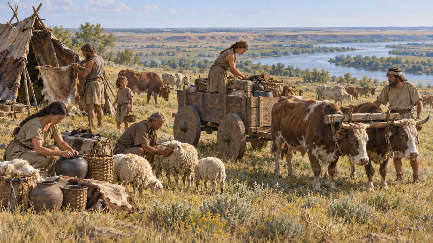
Illustrative reconstruction generated with AI. Lower Don–Volga region, around 3000 BCE. Herding, dairy products and wagon transport have archaeological and biomolecular support; the camp, garments and faces are illustrative choices rather than an exact reconstruction. References: Wilkin et al., 2021 and the 2022 study of dairying in the Caucasus and Eurasian steppes.
At Castillejo del Bonete, in Terrinches, Ciudad Real, two people were buried beside each other during the Bronze Age. The position of their bodies did not reveal where their ancestors had lived. DNA added an invisible difference: the man had ancestry related to central European groups; the woman resembled the Iberian population before that arrival. Sharing a grave does not establish that they were a couple or allow us to reconstruct their biographies. Yet the case opens a window onto a changing world. It appears in Olalde and colleagues’ 2019 study and is discussed by Harvard Medical School.
How do we reconstruct a migration five thousand years ago when nobody wrote down who arrived or where they came from?
There is no marker that says “this person was an immigrant”. The answer requires connecting burials, objects, dates and thousands of genomic positions. Each piece addresses a different question. Archaeology places a life within a location and a society; radiocarbon estimates when it occurred; genetics compares biological relationships; computing makes millions of fragmentary observations manageable.
Four words need to stay separate from the outset. An archaeological culture groups recurring material features: pottery, houses and burial practices. Genetic ancestry describes relationships of descent estimated by comparing DNA. A language is transmitted socially and can change without the replacement of an entire population. Identity concerns how people understand and organise themselves, something that cannot be read directly from a bone. These four things can be related; none automatically equals another.
Before the steppe: Europe had already changed
European hunter-gatherers did not constitute a uniform population. The end of the ice ages and subsequent millennia had brought movements and regional differences. “Western hunter-gatherer” is a useful comparative genetic category, not the name of a people that remained unchanged from Portugal to Poland.
Iberian Mesolithic communities used different resources: forests, coasts, rivers and estuaries. The Muge shell middens in Portugal preserve accumulated shellfish remains, fish and terrestrial animal bones, stone tools, hearths and burials. Those deposits were more than rubbish: they record repeated occupation and activities that can be studied layer by layer. The ICArEHB research portal documents the estuarine setting and the diversity of the local economy.
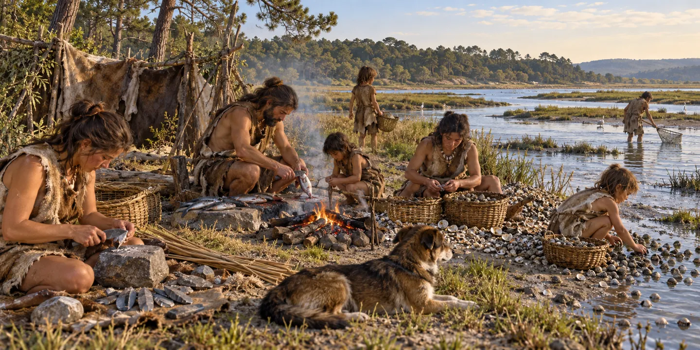
Illustrative reconstruction generated with AI. Muge valley and lower Tagus, around 6000 BCE, inspired by the Mesolithic shell middens. Fishing, shellfish gathering, hearths, stone tools and dogs are supported by the record described by ICArEHB. The camp arrangement, shelter, baskets and garments are illustrative approximations. This is neither a mapped ancient coastline nor a particular excavated dwelling.
Long before steppe ancestry appeared, farming expansion had transformed Europe. Communities related to early farmers in Anatolia and the Aegean spread into the Balkans and onwards through continental and Mediterranean connections. By around 5600 BCE, farming was established in both Iberia and central Europe. Ancient DNA showed that this process involved substantial movements of people: it was more than local groups copying a technique. Mathieson et al.’s study of southeastern Europe reconstructs that context.
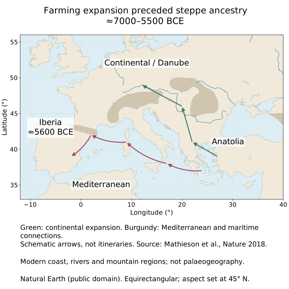
Farming expansion, approximately 7000–5500 BCE. Schematic arrows summarise connections, not individual journeys or exclusive routes. Modern cartography from Natural Earth, public domain; historical source: Mathieson et al., 2018. Coastlines, rivers and mountain regions are modern references without a palaeoclimatic reconstruction. Select the map to enlarge.
Incoming and earlier communities mixed at different rates and in different proportions. Europe did not remain permanently divided between farmers and hunters. By the Iberian Chalcolithic—the Copper Age—its inhabitants already descended from combined histories. We can statistically describe part of that ancestry using ancient samples as references. Doing so does not turn model components into three original peoples coexisting without admixture.
This distinction also matters for the word “Anatolian”. An ancestry component related to Neolithic Anatolian farmers does not imply that a Copper Age individual’s parents were born there. It describes an inherited affinity after centuries of expansion, reproduction and contact.
Yamnaya: livestock, wheels and open geography
Yamna, usually called Yamnaya in the international literature, refers to an archaeological horizon of the Pontic–Caspian steppe, north of the Black and Caspian seas, approximately 3300–2500 BCE. Pit burials under mounds, or kurgans, are among its most recognisable features. Its cultural distribution extended far beyond its initial core: the next map highlights that setting rather than a political border or its entire maximal extent. Lazaridis et al.’s 2025 study revisits its formation and expansion.
Cattle, sheep, wagons and the use of animal products helped sustain mobile ways of life. A wagon allows tools, containers and belongings to be transported beyond what someone could carry on foot. Milk and dairy products provide food without repeatedly slaughtering animals. Identifying milk proteins in dental calculus—the mineralised plaque that can preserve molecules from food—offers evidence independent of human DNA. Wilkin and colleagues documented an important shift in dairy consumption at the beginning of the steppe Bronze Age.
That combination should not become a universal scene of nomads on horseback. Mobility varied with region, resources and community practices. A study of diet and subsistence in the steppes and northern Caucasus shows why local contexts matter. Finding horses does not establish that they were ridden or pulled wagons. The large-scale expansion of the main lineage of present-day domestic horses occurred substantially later than the earliest Yamnaya movements, around 2200 BCE, according to a 2024 analysis of horse genomes.
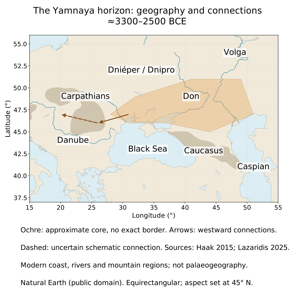
Yamnaya setting, approximately 3300–2500 BCE. Ochre shading approximates the geographical core without precisely delimiting a culture. Arrows indicate western connections; the dashed line emphasises that no exact itinerary is known. Rivers, coastlines and mountain regions: Natural Earth, public domain, modern references without elevation data or palaeocoastlines. Context: Haak et al., 2015 and Lazaridis et al., 2025. Select to enlarge.
Geography helps us formulate possibilities. Major rivers connected steppe, forest and farming environments. The Dnieper—Dnipro—the Don and the Volga structured areas of interaction; the lower Danube and Carpathian Basin opened connections towards central Europe. Mountains could make some movements harder and concentrate them in passes and valleys. None of these features dictates a unique route. A plausible geographical corridor does not prove that a particular family used it.
Reaching Iberia took generations
The signal found in Iberia does not demonstrate a direct journey by an unchanged Yamnaya people from the steppe to present-day Spain. Centuries, intermediate populations and further admixture can separate the formation of an ancestry profile from its appearance in another region.
In 2015, Haak et al. demonstrated a strong genetic relationship between Yamnaya samples and individuals associated with Corded Ware in Germany. In their sampled group, the latter could be modelled with around 75% steppe-related ancestry. That figure belongs to those samples and that model; it does not define everyone who used Corded Ware pottery. The finding supported major demographic movements towards central and northern Europe during the third millennium BCE.
Corded Ware takes its name from decorations made with cord impressions. The later, partly overlapping Bell Beaker phenomenon includes characteristic vessels and other material practices distributed across much of Europe. These archaeological assemblages provide context but are not interchangeable genetic labels.
Olalde et al.’s 2018 Beaker study showed that similar material traditions could spread through different processes. Individuals in Iberian and central European Beaker contexts did not necessarily have the same ancestry. Cultural transmission mattered strongly in some regions; elsewhere, moving people left a very large genetic signature. Carrying a vessel and having descendants in a new place are different processes, even when they coincide.
Moreover, Papac et al.’s 2021 sampling in Bohemia identified changes within Corded Ware and Beaker-associated groups themselves. There was no immutable intermediate population bridging all of Europe. Regional evidence reveals successive contacts and reorganisations that disappear when we draw a single arrow between opposite ends of the continent.
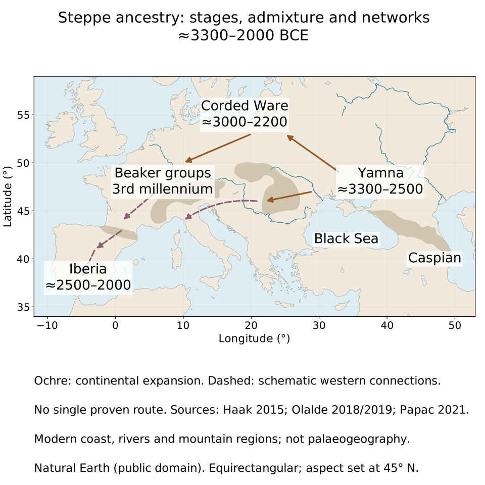
Stages and networks, approximately 3300–2000 BCE. Labels identify archaeological contexts with varying regional chronologies, not genetically pure peoples. Dashed western connections do not select a proven route, nor make every Mediterranean connection a demonstrated entry route into Iberia. Modern base: Natural Earth, public domain. Sources: Haak 2015, Olalde 2018, Olalde 2019 and Papac 2021. Select to enlarge.
For Iberia, comparison with a central European Beaker group is useful because those individuals already had mixed ancestry. But a statistical reference is not a certified geographical departure point. If the actual source group has not been sampled, a similar group may serve as a proxy. We therefore need to distinguish the best available source in a model from the specific ancestors who actually arrived.
A farming peninsula in transformation
Third-millennium BCE Iberia was not empty land awaiting farmers or herders. Communities had fields, flocks, exchange networks and different ways of organising houses and burials. Los Millares in Almería illustrates the complexity of some Copper Age settlements, with defensive enclosures and an extensive cemetery. Its occupation dates approximately to 3200–2200 BCE, according to the site’s documentation from the Junta de Andalucía.
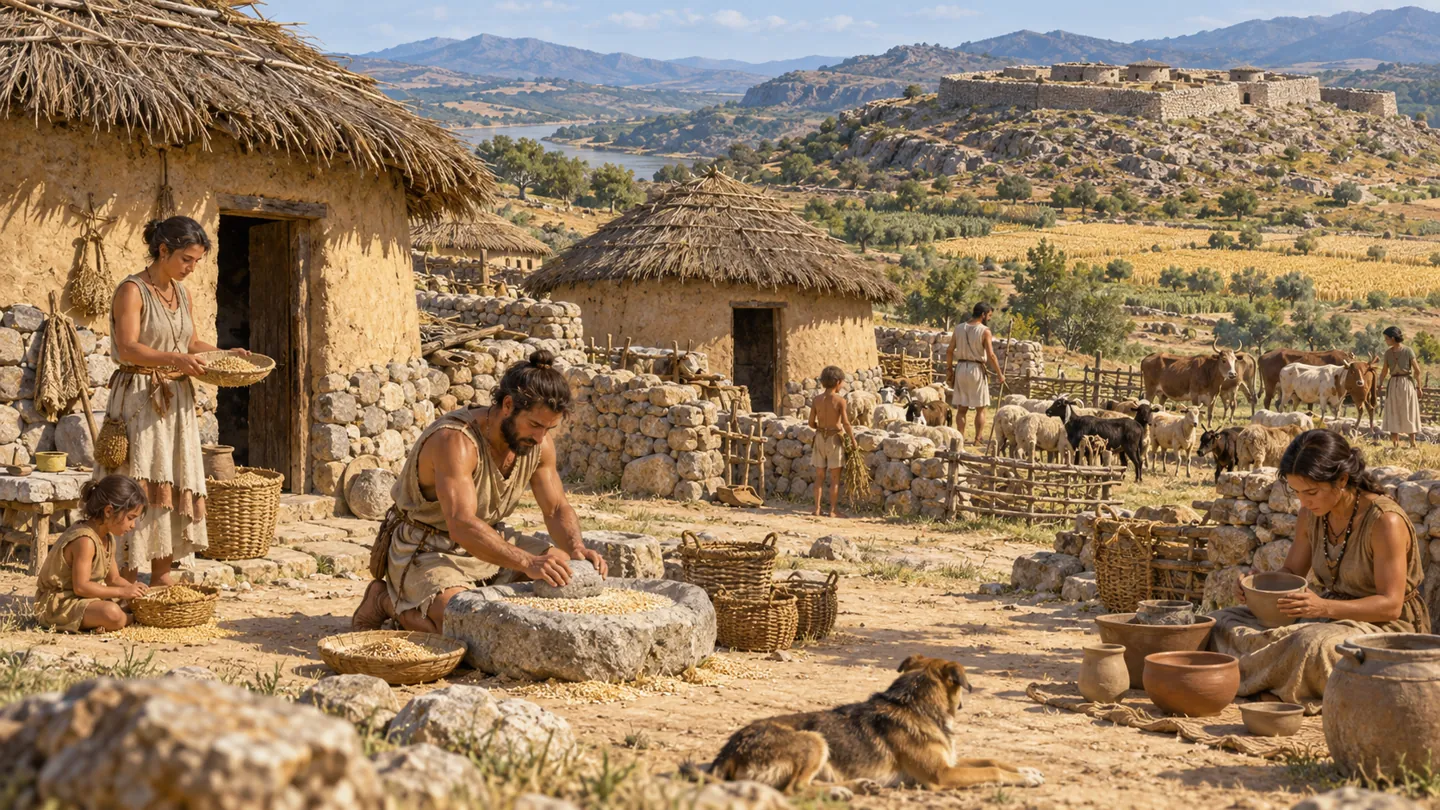
Illustrative reconstruction generated with AI. Southeastern Iberia, around 2800 BCE, inspired by Los Millares. Circular domestic architecture, farming, herding and crafts provide the framework; roofs, clothing, settlement arrangement and the distant enclosure are illustrative choices. This is not an exact reconstruction of an excavated phase.
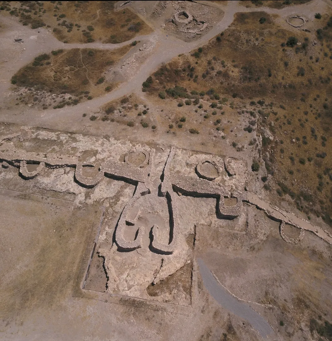
Main gate or barbican at Los Millares, viewed from west-southwest. Photograph by Eamand, 31 October 2017; original and authorship, CC BY-SA 4.0. Resized and converted to WebP; this adaptation retains the licence. This is an Iberian Copper Age site, not a Yamnaya site.

Steppe ancestry appearing in late Copper Age and Bronze Age Iberian samples represents a change within that earlier history. It did not unfold identically across the peninsula. The earliest people detected with that ancestry could live alongside others without it; subsequent generations show admixture. Dates and sample distribution are needed to distinguish an initial arrival from diffusion and later contacts.
The 2019 study, combining 271 newly reported Iberian individuals with previously published data, constructed an eight-thousand-year sequence. Iñigo Olalde was first author; Carles Lalueza-Fox and David Reich were corresponding authors alongside him. The research depended on an international collaboration of archaeologists, anthropologists, collection specialists, laboratory scientists and analysts. Excavations and knowledge of each context were essential to making molecular observations interpretable.
What does “40%” actually mean?
In table S11 of the 2019 supplement, Iberia_BA is modelled using two sources: Iberia_CA, related to the local Copper Age population, and Germany_Beaker, a German Beaker-associated reference. The estimated contribution of the latter is 39.6%, with a standard error of 1.0 percentage point.
This estimates the sampled group’s autosomal ancestry under that model. It does not count immigrants in a village or people who died. Nor does it mean “40% Yamnaya DNA”: the immigrant source proxy already incorporated ancestry from European farmers and hunter-gatherers as well as steppe-related ancestry.
An invented arithmetic example helps: if a source had 50% steppe ancestry and contributed 40% to another population, it would contribute 20% of that component. These figures are pedagogical, not a new calculation from the study. The operation explains why “contribution from incoming groups” and “steppe ancestry” are different quantities. Changing sources, periods or regional samples can also change the estimate.
What does Y-chromosome turnover mean?
Section SI 5 reports 30 Iberian Bronze Age males with sufficient coverage to assign R1b-M269: all 30 belonged to that branch. Within the subset with further resolution, 15 of 15 could be classified as R1b-P312. This supports the almost complete Y-lineage turnover described relative to earlier sampled groups; it does not certify that every man throughout Iberia carried the same lineage.
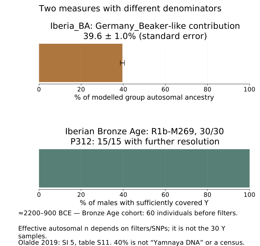
Two different denominators. Above: coefficient in the autosomal model Germany_Beaker + Iberia_CA → Iberia_BA, with ±1 standard error, not a direct percentage of Yamnaya ancestry. Below: observed frequency among males with sufficiently covered Y chromosomes. The study assembled 60 Iberian Bronze Age individuals before filtering—53 new and seven published. The effective autosomal sample size depends on admitted individuals and available SNPs in each analysis and is not the 30 Y samples. General period: approximately 2200–900 BCE; this is not a census around 2000 BCE. Source: Olalde 2019, SI 4–5 and table S11. Original figure; select to enlarge.
The measures describe different things. A population can retain substantial earlier autosomal ancestry while its paternal lineage frequencies change dramatically. Understanding how requires a closer look at inheritance.
A haplogroup is a branch, not a biography
Human DNA is organised into chromosomes. In the most common chromosomal arrangement, a person has 22 pairs of autosomes, alongside sex chromosomes. One copy of each autosome comes from each parent. During egg and sperm formation, copies exchange segments through recombination. Autosomes therefore combine pieces from many family branches.
The Y chromosome usually passes from father to son. Much of it—outside the regions that can recombine with X—retains paternal transmission without the recombination that reshuffles autosomes. Changes in sequence, or mutations, accumulate over generations. An inherited change can serve as a marker for descendants of the same line.
A haplotype is a combination of variants in a region or sequence. A haplogroup groups lineages sharing mutations derived from a common ancestor. Accumulating markers allows a tree to be built: a broad branch contains younger subdivisions. Naming a marker such as M269 or P312 is often preferable to relying solely on a long alphanumeric label, since nomenclature changes as the tree improves.
Mitochondria are cellular structures with their own small genome. Mitochondrial DNA is normally inherited maternally: mothers pass it to sons and daughters, and continuity across generations is traced through daughters. It offers another uniparental line. Neither mitochondrial DNA nor Y represents someone’s entire genealogy.
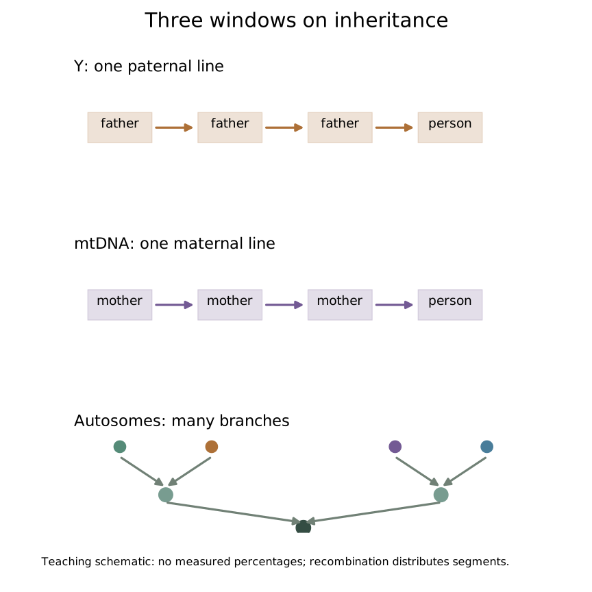
Original teaching schematic of usual inheritance. The autosomal panel illustrates branches and recombination, not measured percentages or a complete pedigree. Methodological references: Olalde 2019, SI 5 and HaploGrep. Select to enlarge.
Imagine a man who has only daughters. His Y chromosome does not continue through them. Part of his autosomal DNA does, and may persist in later generations. The disappearance of a Y lineage therefore does not imply the disappearance of all ancestry from its carriers.
Tree resolution also matters. Among the Core Yamnaya samples in the 2025 study, 49 of 51 Y assignments were R-M269 and 41 of 51 were the subbranch R-Z2103. The 2019 Iberian Bronze Age samples predominantly received R1b-M269 assignments and, where further resolution was possible, R1b-P312. P312 belongs to the western L51 branch; Z2103 is another branch beneath their shared ancestor L23. Sharing R1b or M269 does not make those lineages identical.
The Iberian supplement also documents evidence of DF27 in some males but warns that recovery of the marker was poor: failing to read a position is not the same as testing negative for its mutation. The 2021 southern Iberian study adds resolution on R1b-Z195, within DF27. The southern pre-Bronze Age group includes I2a, G2a and H2; the new Bronze Age samples also contain a non-R1b-M269 exception, a subadult from La Bastida assigned to E1b1b1a1b1. Yamnaya diversity matters too: the 2025 Don group is dominated by I-L699 (17 of 20 assignments), unlike Core Yamnaya. Sublineages and coverage constrain hypotheses; by themselves they do not identify a culture, language or identity. 2021 supplement, section 3 and Lazaridis 2025.
Dates before arrows
Two genetically similar skeletons might be separated by two thousand years. Without chronology, comparison could confuse a possible ancestry source with its descendants. A temporal sequence makes the difference between observing similarity and reconstructing a process.
Radiocarbon dating relies on carbon-14 incorporated during life decaying after death. Measuring its abundance in appropriate material, such as preserved bone collagen, yields a radiocarbon age. Material must be cleaned and assessed so that the measurement relates to the bone rather than adhesives, sediments or other contamination.
That age is not yet a calendar year. Atmospheric carbon-14 has varied, so measurements are compared with a calibration curve built using material of known age. The result is usually an interval, sometimes containing several probability ranges. Reservoir effects—for example, from particular aquatic dietary resources—can shift dates and need specific assessment. OxCal’s documentation explains its calibration and chronological modelling software.
The 2019 study added 26 direct dates. Its supplement distinguishes dates obtained from the human remains themselves from ages assigned using archaeological context, and specifies OxCal 4.2.3 and IntCal13 as its historical calibration tools. This is not a recommendation to use that curve today for any project. Contextual dating can be useful but often requires more caution: graves can be reused, bones displaced, and an object need not have the same age as every adjacent human remain. Supplement, SI 1–2.
From bone to comparable data
Ancient DNA does not arrive in the laboratory as a complete human sequence. Fragments are often short, scarce and chemically altered; microbial DNA and modern contamination can coexist with them. Heat, moisture, soil, burial practices and subsequent conservation influence what survives. The petrous part of the temporal bone and teeth may preserve useful DNA, but sampling remains an intervention on human remains requiring permission and archaeological judgement.
A sequencing library consists of fragments prepared with adapters and identifiers so that a machine can read them. Sequencing produces reads: short base sequences accompanied by quality measures. Researchers then need to determine which reads belong to each sample, which are reliable enough and where they fit.
A SNP, or single-nucleotide polymorphism, is a position where single-base variants occur. If some individuals have A and others G at a location, those versions are alleles. Comparing a shared set of positions produces manageable matrices without reconstructing every complete genome.
The Iberian study enriched libraries for approximately 1.2 million positions in the 1240k panel, plus the mitochondrial genome. Enrichment favours selected fragments using probes: it is not unselected sequencing of all DNA from a bone. Libraries underwent partial UDG treatment, an enzyme procedure that reduces much uracil-associated damage while retaining terminal signals useful for authenticity checks. Details appear in SI 3 of the supplement.
Prepare, align and avoid counting the same molecule twice
Tools in the historical pipeline had specific jobs:
| Step | Tool or procedure documented in 2019 | Problem addressed |
|---|---|---|
| Prepare reads | SeqPrep, modified version 1.1 | Trim adapters and merge overlapping reads from opposite ends of the same fragment. |
| Locate fragments | BWA 0.6.1, using samse; nuclear reference hg19 | Align sequences to comparable coordinates; mitochondrial DNA was aligned to RSRS. |
| Remove repeated copies | Deduplication using alignment coordinates and orientation | Amplification produces multiple reads from a single molecule; these should not be treated as independent observations. |
| Assess contamination | contamMix 1.0.10 and ANGSD | Examine mitochondrial mixtures and estimate X contamination in males with sufficient data. |
| Classify lineages | HaploGrep2 for mtDNA; filtered Y markers | Compare inherited mutations with reference trees while respecting available resolution. |
Historical pipeline: Olalde 2019, SI 4–5. Software websites provide documentation, not evidence that their current versions were used.
Alignment does not discover where someone was born. It answers a prior question: “Which genomic position does this fragment correspond to?” A short read may fit several locations, and a reference can introduce bias. Quality filters help limit these problems. Y assignments required mapping and base qualities of at least 30.
Contamination asks another question: “Are we measuring the buried person or some DNA from people who handled the remains?” In a male carrying a single X, unexpected differences between reads from that chromosome can help estimate contamination. This is not an infallible detector and requires sufficient coverage. It is combined with other checks, including characteristic ancient-DNA damage and mitochondrial consistency.
Low coverage: one observed base is not two known copies
Coverage describes how many times a position is read. An autosome has two copies, but with few fragments we may observe only one. Turning a single A read into a diploid AA genotype is risky: the other copy could be G.
For many comparisons, the study used a pseudohaploid representation: at each covered position, one read was chosen randomly and its observed allele recorded. The person still had two copies; the matrix retained one observation per position. This makes samples with unequal coverage easier to combine, at the cost of losing heterozygosity information and introducing sampling noise.
When there is no read, the value is missing. It does not mean “ancestral allele”, “zero ancestry” or “identical to the reference”. Analyses must handle these gaps explicitly. The 2019 study required at least 10,000 covered SNPs for genome-wide analyses and trimmed read ends according to damage treatment. Main findings were also checked after removing CpG positions susceptible to residual errors. SI 4 and 7.
A grave containing siblings is not two independent samples
Kinship can be investigated by comparing shared or differing variants between individuals. With low-coverage data, uncertainty and background diversity need to be considered. The study identified the two La Braña individuals as brothers using autosomal comparisons, their uniparental lineages and shared X segments. SI 6.
That relationship was an interesting result but also a sampling issue. If five siblings are treated as five independent people, a family can artificially dominate a population’s position. First-degree relatives were therefore excluded from certain genome-wide analyses, retaining the better-covered individual. For investigations of family organisation, however, those relationships are exactly the evidence of interest.
From a large matrix to historical questions
A genetic matrix can have individuals as rows and variants as columns. With complete diploid data, a cell can record 0, 1 or 2 copies of an allele. In a pseudohaploid representation, it records a single sampled base. The number entered depends on available observations, not only on the biology we want to understand.
PCA: a map of variation, not migration
Principal component analysis, or PCA, finds combinations of columns summarising variation between rows. Its first axis captures the largest possible variation under the chosen preprocessing; its second captures the largest remaining portion expressible in a direction perpendicular to the first. Reducing thousands of dimensions to two makes affinities, gradients and unusual samples easier to see.
Axes are not countries, dates or ancestry percentages. They also depend on included individuals, selected variants and data handling. Nearby points may share history, but proximity does not itself demonstrate a migration, its direction or its date. For the method, see Patterson, Price and Reich, 2006.
The 2019 study used smartpca, part of EIGENSOFT: axes were computed from present-day individuals, with ancient individuals projected onto them using options to handle projection and shrinkage. This was not simply filling every gap and recomputing PCA jointly on all individuals. Supplement, SI 8.
A small, entirely synthetic demonstration
The following figure uses 12 fictional individuals and 18 invented variants, without historical population labels. Frequencies change smoothly between individuals with random variation: no pure blocks were created. Of 216 cells, 36 are missing. This demonstrates algebra; it neither reproduces nor provides evidence for the Iberian study.
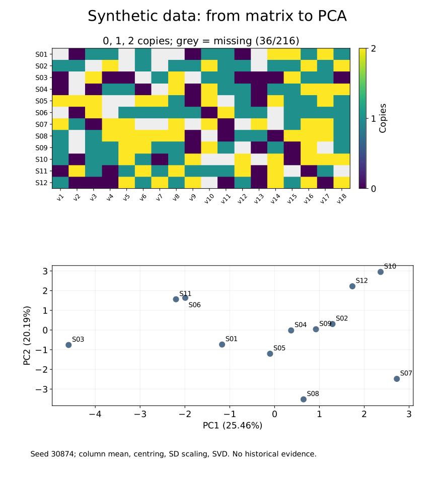
Synthetic data. Seed 30874; diploid genotypes 0/1/2, random missingness independent of genotype, column-mean imputation, centring and sample-standard-deviation scaling after imputation, removal of invariant columns and SVD decomposition. PC1 summarises 25.46% and PC2 20.19% of the processed matrix’s variation. Original demonstration, not the 2019 PCA. CSV data, complete executed script and numerical output. Select to enlarge.
Once matrix M has been constructed, the core computation is short:
# Synthetic diploid example, NOT an ancient-DNA pipeline.
means = np.nanmean(M, axis=0)
filled = np.where(np.isnan(M), means, M)
centered = filled - means
sd = centered.std(axis=0, ddof=1)
Z = centered[:, sd > 0] / sd[sd > 0]
U, s, Vt = np.linalg.svd(Z, full_matrices=False)
scores = U[:, :2] * s[:2]
Mean imputation keeps the computer from trying to treat a missing observation as an observed number; it also brings that cell towards the centre and can distort structure. This is an explicit decision for a teaching toy, not a recommendation for ancient-DNA analysis. The complete NumPy script checks centring, scaling, finite values and SVD reconstruction of the matrix. Reversing an axis sign would reflect the figure without changing its mathematical content.
f4 statistics: explicit affinity comparisons
A visualisation suggests questions; a statistic helps test them. f4 statistics compare differences in allele frequencies between four populations. Schematically, they average (pA − pB) × (pC − pD) over many variants, where each p denotes an allele frequency.
If differences between A and B systematically covary with differences between C and D, the statistic may differ from zero. Under an appropriate tree history, a null expectation helps investigate affinities that the tree cannot explain. The sign changes when population order changes. A deviation must be interpreted against the model and alternatives: it does not encode a unique migration direction or a complete narrative. Patterson et al., 2012.
Olalde et al. calculated f4 using qpDstat in ADMIXTOOLS, with f4mode: YES. This is a specific option: f4 and a related D statistic are not interchangeable values. The official qpDstat documentation describes the distinction.
qpAdm: compatible admixture is not the only true history
qpAdm tests whether a target population can be represented as a combination of sources in its relationships to a set of reference populations. References must distinguish sources sufficiently; they need not be completely disconnected spectators to the entire history. Choice of sets and unmodelled relationships affect the result.
The program estimates mixture coefficients and evaluates constraints on a matrix of f4 statistics. Results may show that a single source is insufficient or that two sources are compatible. But sources are often proxies: sampled individuals representing genetic relationships, not necessarily the exact historical ancestors.
A high p-value does not mean “there is a 90% probability that this history is true”. Under the test’s assumptions, it means that the observed discrepancy is not strong enough to reject those constraints with the available data. Multiple models can pass. Limited sampling, similar sources or continuous gene flow may prevent them from being distinguished. Harney et al.’s 2021 evaluation and its supplementary guide explain these limitations.
In Iberia this approach helps separate a local Copper Age source from an incoming source that was already mixed. The 2019 supplement warns that attributing all European Neolithic-related ancestry to local people is inappropriate: incoming steppe-related groups also brought some of it. A “local Iberians + Yamnaya” mixture can therefore be an inadequate simplification.
Uncertainty: a million observations are not a million independent tests
Nearby variants may be inherited together, so treating them as independent observations would underestimate error. The block jackknife divides the genome into blocks and repeats a calculation while leaving out one block at a time. Variation between those estimates yields standard errors that account for some of this dependence.
The 2019 study used 5-megabase blocks for f4 and 10-megabase blocks in its specific X/autosome comparison. A megabase is a million positions. Block size, coverage and the number of available regions matter. An error bar describes statistical uncertainty under the analysis; it does not automatically capture every archaeological bias or possible history. SI 9 and 11.
Men, women and what a paternal signal cannot tell us
Steppe ancestry occurs in both men and women. The Y chromosome observes one paternal line; it cannot establish that new ancestry was restricted to males.
To investigate sex differences in contributions, researchers compare X with autosomes. In the usual arrangement and a simple balanced-sex model, women carry two X chromosomes and men one. Around two-thirds of X copies come from mothers and one-third from fathers. Autosomes receive equal contributions from both parents. A strongly male-biased immigrant contribution can leave less source-related ancestry on X than on autosomes.
This comparison is not a direct count of travelling men. It depends on admixture sequence, chosen sources, elapsed time and uncertainty. In 2019, the contrast suggested less Germany_Beaker-like ancestry on X, with Z = 2.64 and broad errors. That signal accompanied much more striking Y turnover. Together they supported a sex-biased contribution interpretation, without specifying a unique social mechanism. SI 11, table S14.
Villalba-Mouco et al.’s 2021 southeastern study, focused especially on El Argar societies, did not detect significant male bias in steppe ancestry through its X/autosome models. The 2025 Portugal study likewise did not detect it in its Bronze Age groups. This prevents paternal patterns from becoming an identical rule for all Iberia. Failure to detect a difference does not demonstrate that it never existed: later samples may record already balanced admixture, and X offers less information.
Social hypotheses include founder effects, patrilineal organisation—affiliation or status transmitted through the paternal line—patrilocal residence—living near the man’s group—differences in reproductive success and successive migrations. These processes may act together. They need testing against kinship, burial distribution, isotopic mobility and settlement archaeology.
DNA does not automatically imply massacres, expulsions or military conquest. Nor does it reveal women’s personal preferences or specific family agreements. Violence can be investigated where injuries and contexts document it; it is not the necessary translation of a haplogroup chart.
What research refined after 2019
Subsequent research makes the original result more regional, more chronological and more demanding in its interpretation, rather than turning it into a final snapshot.
Southeastern Iberia, 2021. Villalba-Mouco and colleagues studied 136 individuals, 122 of whom contributed data for more detailed population analyses. Their sequence connects the spread of steppe ancestry into the south with the transition around 2200 BCE and the emergence of El Argar, while investigating kinship and social organisation. Y turnover is pronounced; family relationships are compatible with patrilineal organisation and female exogamy, without making those practices universal across every household. Mediterranean affinities also require consideration of more than one external contribution. Article and additional materials.
Portugal, 2025. Roca-Rada et al. expand the history of the western peninsula and demonstrate differences between groups and models. They report low levels of steppe affinity in certain Beaker contexts, wider spread during the Bronze Age and local persistence. As discussed above, paternal lineage turnover and X/autosome comparisons do not deliver precisely the same conclusion. Genome Biology.
The northeast, 2025–2026. The Los Castellets II study examined 24 Late Bronze Age adults and identified numerous relatives: another warning against treating a funerary collection as a random sample. Its analyses suggest a regional increase in steppe ancestry, but some comparisons fail to reach statistical significance. A 2026 Iron Age study obtained genome-wide data from 22 individuals out of 54 newborn burials and documented continuity with Bronze Age-derived populations alongside subsequent changes. These are regional and socially selective windows, not substitutes for the whole peninsula. Los Castellets II and the Iron Age study.
The origins of Yamnaya themselves, 2025. Lazaridis, Patterson, Anthony and a large international collaboration place their formation within earlier admixture networks linking the Caucasus, lower Volga and Dnipro–Don populations. A model of an original pure steppe population becomes even less appropriate. The study also proposes connections to Indo-European language expansion, but DNA does not preserve someone’s spoken language: that reconstruction requires additional linguistic and archaeological arguments. Nature, with supplement and tables.
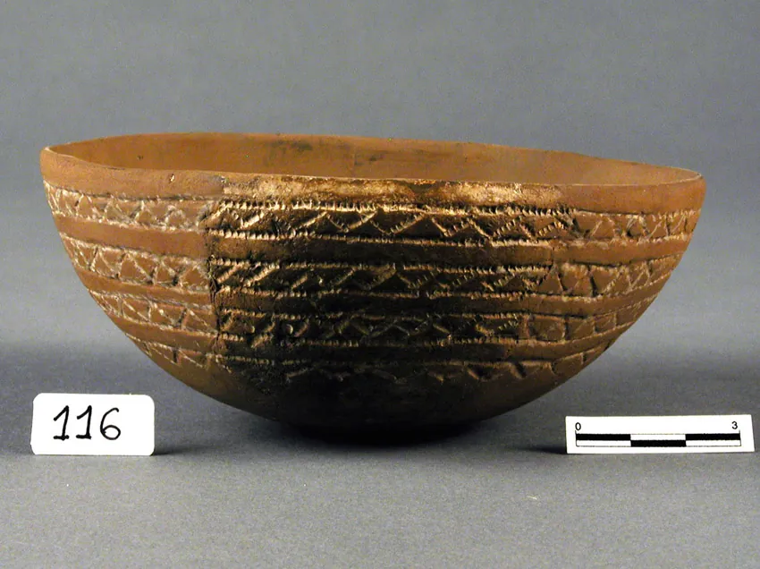
Bowl from the Los Millares society, Museo de Almería. Photograph and own work by Museo de Almeria according to the original record; CC BY-SA 3.0. Converted to WebP under the same licence. The object belongs to an Iberian Copper Age context; it is not presented as Yamnaya pottery or a genetic marker.

A collection of burials is not a census
Preservation determines which lives can be studied. A warm region may yield less DNA than another; cremation may destroy it; a cemetery can concentrate a social group; excavations may recover some phases better than others. Technical filters then select samples suitable for particular analyses.
This has two consequences. Presence is an observation: a signal has been found in a person of a particular context and date. Absence from samples does not guarantee absence from the entire population. A frequency within a collection should not automatically become the frequency among millions of unsampled people.
Models have limits too. An unsampled ancestral group can resemble an available source. Different histories can produce similar affinities. More coverage improves knowledge of an individual but does not itself fix biased geographical sampling. More individuals help, but a hundred relatives from one cemetery do not represent a hundred independent communities.
The strongest inference combines methods that fail in different ways: direct dates, stratigraphy, autosomal DNA, lineages, kinship and isotopic mobility evidence. Agreement on a compatible process increases confidence; disagreement may point to a more complex history or an issue needing review.
What role did machine learning play?
PCA belongs to the repertoire of unsupervised learning: it extracts structure without receiving each individual’s “true origin” label. It is also a classical statistical technique. Calling it machine learning can be correct; presenting the whole research programme as artificial intelligence would obscure the actual tasks and assumptions.
For the central 2019 results, visual exploration used PCA, while affinity and admixture hypotheses were tested with f statistics and qpAdm. The sources do not attribute those conclusions to neural networks. Read alignment, contamination estimation, haplogroup classification and statistical testing do not become the same operation because they run on a computer.
Current tools can support reproducible pipelines and new analyses, but they must be distinguished from historical software. For learning today, consult ADMIXTOOLS, EIGENSOFT or ADMIXTOOLS 2. We have not reanalysed the Iberian genomes using their current versions or replaced published results with the synthetic example.
Returning to the fragment supporting the story
The ENA deposit PRJEB30874 provides access to study sequences. Its file report lists FASTQ reads and submitted BAM files with BAI indexes. FASTQ stores sequences and qualities; BAM organises aligned reads. This is not a ready-made table of interpreted ancestry percentages. Comparative matrices, identifiers, dates, reference sources and filters remain necessary to reproduce an analysis.
Being able to move from a claim back to its data is one of computing’s decisive contributions. It does more than accelerate arithmetic: it allows observations to be organised, tests repeated, proxy sources changed and conclusions checked against those choices. A reproducible number still needs responsible historical interpretation.
The people at Castillejo del Bonete left no record of their ancestors. Their bones incompletely preserve fragments of relationships connecting them to other humans. Comparing those fragments with remains from different places and dates reveals that the Iberian Bronze Age transition included profound demographic movements and lasting admixture. What we cannot yet write with equal confidence is one collective biography: who took each route, what families negotiated or why some lineages had more descendants than others.
The opening question therefore has a precise answer: we reconstruct migration by comparing dated fragments, testing models and defining what the data cannot resolve. Computers make a previously inaccessible signal detectable. Archaeology reminds us that the signal comes from lives, not blocks of colour.
Bibliography and resources
- Olalde, I., et al. (2019). “The genomic history of the Iberian Peninsula over the past 8000 years”. Science, 363, 1230–1234. DOI: 10.1126/science.aav4040, open text, supplement: contexts, laboratory and methods SI 1–11; tables S11–S14.
- Haak, W., et al. (2015). “Massive migration from the steppe was a source for Indo-European languages in Europe”. Nature, 522, 207–211. DOI: 10.1038/nature14317, open text, supplement.
- Olalde, I., et al. (2018). “The Beaker phenomenon and the genomic transformation of northwest Europe”. Nature, 555, 190–196. DOI: 10.1038/nature25738.
- Mathieson, I., et al. (2018). “The genomic history of southeastern Europe”. Nature, 555, 197–203. DOI: 10.1038/nature25778.
- Villalba-Mouco, V., et al. (2021). “Genomic transformation and social organization during the Copper Age–Bronze Age transition in southern Iberia”. Science Advances, 7, eabi7038. DOI: 10.1126/sciadv.abi7038, text and additional materials.
- Papac, L., et al. (2021). “Dynamic changes in genomic and social structures in third millennium BCE central Europe”. Science Advances, 7, eabi6941. DOI: 10.1126/sciadv.abi6941.
- Lazaridis, I., Patterson, N., Anthony, D., et al. (2025). “The genetic origin of the Indo-Europeans”. Nature, 639, 132–142. DOI: 10.1038/s41586-024-08531-5, supplement and tables.
- Roca-Rada, X., et al. (2025). “The genetic history of Portugal over the past 5,000 years”. Genome Biology, 26, 248. DOI: 10.1186/s13059-025-03707-2.
- Harney, É., Patterson, N., Reich, D. and Wakeley, J. (2021). “Assessing the performance of qpAdm: a statistical tool for studying population admixture”. Genetics, 217, iyaa045. DOI: 10.1093/genetics/iyaa045.
- Patterson, N., Price, A. L. and Reich, D. (2006). “Population Structure and Eigenanalysis”. PLOS Genetics, 2, e190. DOI: 10.1371/journal.pgen.0020190. Patterson, N., et al. (2012). “Ancient Admixture in Human History”. Genetics, 192, 1065–1093. DOI: 10.1534/genetics.112.145037.
- Wilkin, S., et al. (2021). “Dairying enabled Early Bronze Age Yamnaya steppe expansions”. Nature, 598, 629–633. DOI: 10.1038/s41586-021-03798-4. Librado, P., et al. (2024). “Widespread horse-based mobility arose around 2200 BCE in Eurasia”. Nature, 631, 819–825. DOI: 10.1038/s41586-024-07597-5.
Sources reviewed in October 2026. Photo credits and licences appear in captions; maps and charts are original creations and base cartography is public domain. AI images are environmental illustrations and are not used as scientific evidence.